法线压缩、向量存储压缩
The bandwidth cost and memory footprint of vector buffers are limiting factors for GPU rendering in many applications.
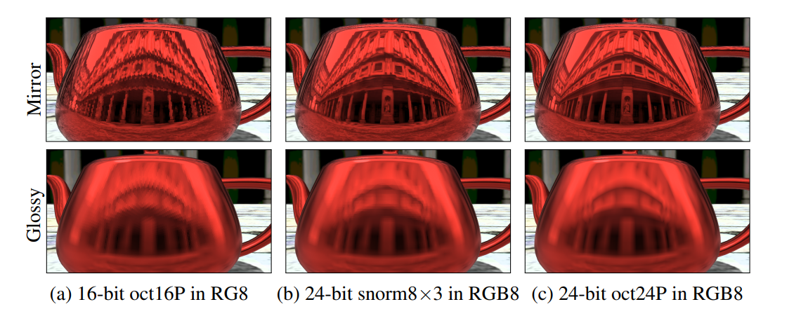
Figure 1. 对几何缓冲区法线存储的选定表示的镜像和光泽反射的影响。
- (a) 16 位 oct16P 方法对典型的 float32×3 法线进行了 8 倍的压缩,尽管有明显的错误。
- (b) 普通的、朴素的 24 位 snorm8×3 表示占用更多空间而没有成比例的改进。
- (c) 24 位 oct24P 表示以与原始方法相同的存储成本极大地提高了精度。
1. Introduction
单位向量在 3D 计算机图形学中无处不在。一些常见的应用是表示表面法线、切线向量和光传播方向。因此,许多图形算法的时间和空间性能取决于读取、处理和写入这些向量的速度。具体来说,访问 attribute streams 和G-buffers(几何缓冲区)所需的带宽以及该数据的内存占用是许多应用程序中 GPU 渲染的限制因素。
游戏开发人员最近的演示展示了最小化带宽和内存占用对于现代 GPU 上的实时应用程序的重要性。这些开发人员已经表现出愿意采用相对复杂的编码和解码方案,并接受因精度损失而导致的可见错误 [Kaplanyan 2010]。例如,电子游戏《命运》目前正在 Bungie 制作中。它将所有用于着色像素的属性——位置、表面法线、材质标志和完整的各向异性 BSDF 参数打包成 96 位——这只是三个标量 float32 值的足迹 [Tatarchuk 等人。2013]。
In a modern graphics pipeline, 3D vectors reside either in high-bandwidth registers, medium-bandwidth DRAM memory buffers (and on-chip caches of them), or some form of relatively low-bandwidth storage, such as local or network disks or SSDs.
The high- and low-bandwidth cases encourage minimizing decode time and storage space, respectively.
寄存器鼓励为通常为 96 位宽的单位向量采用一种简单的、计算友好的存储格式:三个 32 位浮点数表示 x、y 和 z 坐标。我们将这种格式表示为 float32×3。
It exclusively favors computation speed over space.
Disks and networks have low bandwidth compared to on-chip communication pathways. So, those media encourage the most space-efficient format even at the expense of significant computation for encoding and decoding. General geometry compression in the disk and network context was well-explored by Deering’s seminal paper [1995] and work that follows it, e.g., most recently extended for GPUs by Pool et al. [2012].
For unit vectors in medium-bandwidth DRAM and on-chip caches, a combination of speed and space requirements introduces interesting tradeoffs. This is the case that we consider. The bandwidth and latency of accessing in-core memory are orders of magnitude more favorable than the properties of disk or network, but also orders of magnitude less favorable than those of register storage. It is therefore desirable to expend some computation to encode and decode unit vectors between space- and time-efficient representations, but it is also unacceptable to introduce significant error or to expend significant amounts of computation in the process.
DXN/BC5/ATI2/3Dc [ATI 2005] 等专用压缩格式利用法线贴图中空间局部表面法线的统计依赖性来降低带宽和存储成本。法线贴图的压缩是当今实时应用程序的行业标准做法。Such formats have limitations, of course. The error increases with the variance of the normals in a neighborhood, such formats are often too expensive to encode at runtime, and texture map compression is not at all appropriate for unit vectors in attribute streams that have no natural 2D locality.
We survey methods from industry and academia for sets of unit vectors where no statistical dependence can be assumed between elements. Two examples of cases in which this is important include the attributes packed in an indexed vertex array describing geometry, and the surface normals stored in a geometry buffer for deferred shading [Pranckevicius 2010 ˇ ]. Note that it may also be desirable for encode and decode costs to be asymmetric. For example, with static geometry in a scene, one is willing to spend significant offline computation to precompute a space-efficient vertex normal representation so long as that representation can be decoded to float32×3 efficiently at runtime.
1.1. Formal Problem and Intuition
The goal of the surveyed methods is to represent a unit vector using the fewest bits at a given, acceptable representation error, or alternatively to minimize representation error for a fixed bit-width.
This is the problem that integer, fixed-point, and floatingpoint representations address for intervals of the real line, but extended to points on the sphere. Representation error is a necessary condition for digital computation in real-number domains and is pervasive in computer science.
Consider a straightforward representation of points on the unit sphere.
A structure comprising three 32-bit floating scalars (struct { float x, y, z; }) occupies
This representation spans the full 3D real space, \(R^3\) , distributing precision approximately exponentially away from the origin until it jumps to infinity. Since almost all representable points in this representation are not on the unit sphere, almost all 96-bit patterns are useless for representing unit vectors. Thus, a huge number of patterns have been wasted for our purpose, and there is an opportunity to achieve the same set of representable vectors using fewer bits, or to increase effective precision at the same number of bits. From this example, it is obvious that one condition for an ideal representation format is for every possible bit pattern to represent a unique point on the sphere. (There are performance reasons—explored in the next section—for why we might wish to forgo a small number of patterns, but never more than a small constant.)
Spherical coordinates are a natural way to satisfy the requirement that almost all bit patterns correspond to points on the unit sphere.
Indeed, storing two 32-bit floating-point (or fixed-point) angles for a total of \(64 bits / unitVector\) does dramatically increase representation precision, while simultaneously decreasing storage cost. Of course, spherical coordinates require some trigonometric operations to convert back to a Cartesian point for further computation. Those operations themselves introduce error as well as costing time (and power), the kind of tradeoff that we have already motivated. An ideal format would allow for efficient and accuracy-preserving compression and decompression.
When considering all 64-bit patterns interpreted as spherical coordinates, note that the represented unit vectors clump near the poles and are sparse near the equator. This bias is undesirable in most applications. So, an ideal format would furthermore distribute representable points uniformly on the sphere to minimize bias and worstcase representation error.
With these properties in mind, we have several opportunities to capture space, precision, and efficiency that are presented by the geometry of the sphere. Mappings between the sphere and the real square in various dimensions can exploit symmetry [Deering 1995]; for example, positive and negative hemispheres lead to eight reflected octants, within an octant all axes have symmetry, and one can even recurse further if needed. It is tempting to observe that for some applications in graphics (e.g., camera-space normal vectors) only the hemisphere apparently requires representation; however, due to perspective, bump mapping, and vertex normal interpolation many of these applications actually require a full sphere in practice. Furthermore, reduction to a hemisphere would only save a single bit.
For the specific representations surveyed in this paper, we make the assumption that one is encoding a Cartesian float32×3 vector into a compressed representation or decoding such a representation into float32×3. We measure round-trip encode and decode error from a float32×3 input, since that is the additional precision loss of including some encoding in a larger program. However, we note that float32×3 is already an approximation of a real vector, so it is possible that for particular applications the compressed representation may actually be more accurate than the uncompressed one. We further consider the impact of higher-precision intermediate values during the encoding and decoding step, but observe that the impact on precision is slight.
The code listings in the paper are written with the assumption that GPU fixedfunction hardware is available to map between scalar float32 format and various scalar representations discussed in the next section. We believe that this assumption holds for all current GPUs, including mobile parts, for typical power-of-two bit sizes (8, 16, 32) as well as some exotic GPU formats (such as 10- and 11-bit float employed by GL_R11G11B10F, 14-bit fixed point from GL_RGB9_E5, and 10-bit unorm from GL_RGB10). We also evaluate a hypothetical R11G11B10 snorm format, which mirrors the per-channel bit allowance on the existing GL_R11G11B10F format.
Some unit vector representations rely on storage formats that are not natively supported on CPUs or GPUs, such as snorm12. For storage, however, one can pack anything into the bits of an unsigned integer. Thus, arbitrary sizes are possible at the cost of some extra decoding work.
For example, a 12-bit unit vector can be packed with four bits of material flags into a 16-bit unsigned integer texture format. DirectX 9-class GPUs have limited or no integer support, so pure floating-point arithmetic is preferred over integer operations for this bit packing. Even the newest GPUs have more ALU support for floating point than integer, so the all-floating point implementation is also a performance optimization on those machines. Obviously, this could change on future architectures or ones that can overlap integer and floating-point operations, and it is unfortunate that the all-floating point implementation obfuscates some code.
1.2. Scalar Unit Real Representations-标量单位实数表示
uint b: An unsigned integer with b bits, capable of exactly representing integers on [0 , \(2^b −1\)].
fix i. f : Fixed-point representation of an unsigned integer scaled by a constant negative power of two that represents uniformly distributed values on [0 , \(2^i−1\) + ( \(2^f - 1\)) * \(2^{-f}\)] using b = f +i bits total. (There are various notations for this in the literature, some of which use the total bit size instead of the number of integer bits before the decimal place in the name). Fixed point is never used by any of the representations surveyed in this paper, because it cannot exactly represent 1.0 without wasting an entire bit on the one’s place.
float b: The IEEE-754/854 floating-point representation with b bits total; sign, mantissa, and exponent bits vary with b according to the specification.
unorm b: Unsigned normalized fixed point represents the range [0, 1], with exact representations for both endpoints. Reinterpreting the bits of a unormb-encoded number as an unsigned integer i, the encoding and decoding equations for the real number r are [Kessenich 2011, 124]:
- (1) \(i = round(clamp(r,0,1)*(2^b −1)),\)
- (2) \(r = \frac {i} {(2^b −1)}\)
Most GPUs implement these transformations in fixed-function hardware for converting to and from floating point during texture- or vertex-attribute fetch and frame buffer write, so there is no observable runtime cost for reading and writing such values.
scaled and biased unorm b: One can exploit unorm representations to store signed values by biasing and scaling them. To encode a real number \(−1 ≤ r ≤ 1\) in this format, first remap it to unsigned \(0 ≤ \frac {1} {2} (r +1) ≤ 1\), and then encode as a unorm.
This is used in some legacy systems for encoding vectors in, e.g., RGB8 unorm values. Encoding and decoding cost one fused multiply-add instruction (MADD, a.k.a. FMUL) per scalar, but more critically lose unorm’s ability to automatically convert to floating point in texture hardware. This format cannot exactly represent \(r = 0\).
snorm b: Signed normalized fixed point addresses the limitations of scaled-and-biased unorm. Snorm allows two bit patterns to represent the value -1 so that the number line shifts and zero is exactly representable:
- \[i = round(clamp(r,−1,1) * (2^{b−1} −1)),\]
- \[r = clamp(\frac {i} {2^{(b−1)} −1} ,−1,+1 )\]
As previously mentioned, GPUs currently implement snorm reading and writing in fixed-function hardware.
2. 3D Unit Vector Representations - 3D 单位向量表示
This section gives brief descriptions of unit vector representations. We assign each a meaningful and short name for use in our evaluation section. For accuracy and clarity, as well as brevity, those names sometimes differ from the ones under which the representations were originally introduced to graphics. Note that some of these were historically introduced as parameterizations of the sphere, not compression methods, and that some have been overlooked in the scientific literature despite appearing in game developer presentations.
\(L^2\) accuracy of the decoded \((x, y,z)\)-vector can be improved for nearly all representations by re-normalizing the vector using at least float32 precision after decoding. However, that can increase the angular deflection from the represented vector. Thus, we consider projection of decoded vectors onto the sphere to be an application issue, with the best implementation depending on whether the exact unit length or the direction is more important in a given context. We do not include it as part of the decoding.
float×3: Store unit vector (x, y,z) directly in floats. As noted in the introduction, most bit patterns are wasted because they are not the lowest-error representation of any unit vector. This also has lower precision near the centers of octants, rather than uniformly distributing precision over the sphere.
snorm×3: Store unit vector (x, y,z) directly in snorms. Most bit patterns are wasted by this encoding, but it is very fast. Because the length as well as the direction of the vector will implicitly be quantized by this representation, it is necessary to explicitly re-normalize the vector after decoding it to a higher-precision representation (e.g., snorm8×3 → float32×3).
spherical: Store spherical coordinates \(0 ≤ θ ≤ π , −π ≤ φ ≤ π\), mapped to snorm×2 (because a mix of unorm and snorm is not supported by hardware). Note that this differs from Meyer’s implementation[2012], which uses two unorms of equal length to encode the vector within a hemisphere and an explicit extra bit for the choice of hemisphere, throwing away a bit for even-length representations. Uniformly-spaced spherical coordinates are distributed poorly with clumps at poles, and so the representation error is fairly high for large bit counts. Encoding and decoding also require trigonometric functions, which are expensive on some hardware.
cube: Project onto a cube by dividing by the highest-magnitude component, and then store the cube-face index and coordinates within it (i.e., the standard cube-map projection). This is not a particularly desirable encoding, because it is hard to work with, yet still has high error.
The error arises because points are distributed more densely near where the cube vertices project onto the sphere. The awkwardness and inefficiency is because encoding which of the six faces was dominant consumes three full bits (leaving two patterns unused), and packing three bits plus two components into a word wastes another bit for alignment.
The error of this representation is slightly worse than snorm×3 at the same bit size, yet it requires substantially more computation to operate on, so we do not report further results on this representation.
warpedcube [ISO/IEC 2005]: Use cube parameterization except warp the parameter space to more evenly distribute the representable points. This gives slightly better accuracy at the cost of trigonometric operations for the warping. The awkwardness of the odd bit size remains from cube parameterization, and the error is still substantially higher than similar methods that project onto an octahedron instead, e.g., as shown by Meyer [2012].

Figure 2. The latlong indexing scheme shown for encoding vectors with a maximum error of 10◦ to make the regions clear (derived from Smith et al.’s [2012] figure 4). Only a few indices are labelled in the diagram.
latlong [Smith et al. 2012]: Divide the sphere into approximately equal-area latitudelongitude patches (choosing them to minimize the worst-case error), and then number all patches as shown in Figure 2. Store each vector as the index of the patch that contains it. Encode and decode require fetching a 64-bit (for most encoding sizes) value from a lookup table in addition to the vector itself. Smith et al. called this “Optimal Spherical Coordinates,” but it is not optimal among all possible encodings (only among encodings dividing the sphere into latitude-longitude patches); the sphericalrectangular patches are the key idea, so we assign the descriptive name. Note that this method is distinct from the standard latitude-longitude environment map encoding. This method produces the lowest error of all surveyed, but also has a very high encode and decode cost when implemented in software.
oct [Meyer et al. 2010]: Map the sphere to an octahedron, project down into the \(z = 0\) plane, and then reflect the \(-z\) -hemisphere over the appropriate diagonal as shown in Figure 3. The result fills the \([−1,+1]^2\) square. Store the \((u, v)\)-coordinates in this square as snorm×2. We consider this the best overall method: fast to encode and decode, and a near-uniform mapping. These encoded vectors were originally called “Octahedral Normal Vectors (ONV),” but there is no reason to restrict them to normals (and using “normal” to indicate “unit” in this case is confusing), so we call them “oct” to parallel the spherical and cube parameterizations. This representation is intuitive, has nice distribution properties for all bit sizes, is fairly efficient to encode and decode.
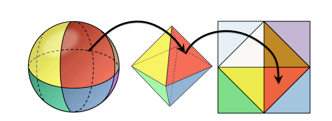
Figure 3. The oct representation maps the octants of a sphere to the faces of an octahedron, which it then projects to the plane and unfolds into a unit square.
and is close to the lowest error for all bit sizes of the representations surveyed. The reason that the mapping is computationally efficient (and elegant) is that it maps the sphere to an octahedron by changing the definition of distance from the \(L^2\) (Euclidean) norm to the \(L^1\) (Manhattan) norm. The first-published reference code had errors at the boundaries due to the use of the sign() function on 0; we correct these in our CPU reference implementation and provide optimized GPU implementations.
stereo (Stereographic), eqarea (Lambert Equal Area), and eqdist (Equidistant) [Snyder and Mitchell 2001]: These use classic cartographic projections to map a hemisphere to a unit-radius disk, using different metrics to minimize distortion. To capture the precision opportunity of the area outside the disk, we extend these projections by mapping the disk to a square with another set of equal-area mappings: concentric [Shirley and Chiu 1997] and elliptical. The latter (which we derived, but is almost certainly not novel) is shown in our supplemental code. Of those classic mappings, eqarea requires the fewest operations, while eqdist, with the elliptical mapping, yields the lowest encoding error.
Meyer [2012] provides the most recent previous survey of unit vector representations. Our survey extends the theoretical results from that thesis by considering more methods, measuring both minimum and maximum error, demonstrating the visual impact under different shading models (for surface normals), measuring encode and decode performance, and providing optimized implementations of the most useful methods.
Pool et al. [2012] present methods for lossless compression of large buffers of arbitrary floating-point data. They reduce the average size of such buffers by at most one third and theorize a slightly better ratio with range compression of the input. We do not recommend this approach for buffers in which the entries are known to be unit vectors. The reason is that knowing the semantics of the data, the methods that we survey achieve strictly better space reductions at improved encoding and decoding performance, with low error rates.
2.1. Bit-length Variants
Each method has precision variants that we parameterize by the total bit size of the output. For example, oct24 stores an snorm12×2 parameterization of the sphere mapped to the unit square by the oct encoding; oct16 stores snorm8×2. As in those examples, almost all representations encode two parameters to which we assign equal bit width. Our notation is designed to build upon the existing scalar notation (e.g., float32) while indicating the total bit width, which is the interesting number from both hardware and software implementation perspectives.
In cases where a biased distribution of points on the unit sphere is desirable, it would be advantageous to assign different precision to different parameters. We are concerned with the general case, in which uniformity is desirable. In that case, it is the encoding’s role to distort the sphere to the given parameter space so that uniform parameter precision gives the best encoding.
There are some exceptions to the uniform dual-parameter space. The raw snormb×3 and floatb×3 formats obviously encode to b bits per parameter for a total of 3b bits. Some formats use extra sign bits to encode which hemisphere/face/octant the remainder of the parameters describe. These have been discussed in the previous work and are unambiguously described by the supplemental code accompanying this paper, better than equations and notation would express in the text.
2.2. Precise Encoding Variants
We define a representation as the semantics of the bit pattern, that is, by the effect of the decoding algorithm. For most representations, there is a natural, relatively fast encoding algorithm that maps float32×3 unit vectors into that format. It is often the case that the fast encoding is incapable of generating certain legal bit patterns, and even when it can, the result can be biased at the final roundoff stage. In these cases, there must also exist some alternative precise encoding algorithm that finds the particular bit pattern that reduces the representation error of the round-trip encoded and then decoded value, compared to the input. The suffix “P” denotes the use of a precise (and necessarily slower) encoding algorithm in our evaluation table.
For snorm×3, the precise encoding algorithm is called Best Fit Normals [Kaplanyan 2010]. It takes advantage of the fact that non-unit vectors normalize to points on the unit sphere inexpressible by unit vectors in snorm format and searches for the non-unit vector that normalizes closest to the desired vector. The search can be reduced to a table lookup of vector lengths, compressed by taking advantage of symmetry. The representation still has a poor distribution of points on the sphere even with the precise encoding. However, the significant advantages of this representation under precise encoding are that one can mix encoded and unencoded normals and that it still has zero decode overhead compared to non-optimized snorm×3, the fastest method for decoding. We evaluate two variants of this algorithm, the first is the exact method implemented by Crytek in the original presentation. This suffers from worse maximum error than any other method we tested, due to the discretization of the lookup table. We refer to this method as CrytekBFN. The second variant, which we refer to as snorm×3P is the precise variant, which tests the four lengths encoded in the closest texels of the lookup table and the original vector, choosing the one that minimizes error. This brings the maximum error down below that of simple snorm×3 encoding and further decreases mean error.
Many methods operate by mapping the real sphere S 2 to the real plane R 2 , and then to a subset of the integer plane Z 2 . There is a small amount of error introduced by the finite-precision floating-point math during the S 2 → R 2 transformation. We consider the impact in practice of using float32 and float64 in the implementation of that mapping for intermediate results. More significant error is frequently introduced by the R 2 → Z 2 mapping. Furthermore, simply rounding to the nearest integer after scaling will produce more and biased error, since each method of unwrapping the sphere necessarily has some asymmetry. Therefore, algorithms that operate by these mappings can be made more precise by choosing between the floor and ceiling operators along each axis based on minimizing round-trip error.
For several representations, the error inherent in the representation was already so much worse than alternatives that precise encoding only made the method undesirably slow without making the quality competitive. To focus this survey on the most attractive methods, we do not report the error difference between precise and fast encoding for such low-quality representations.
2.3. The Precise Decoding Variant of Latlong
We have already discussed precise encoding. The latlong representation has the unusual property that it always requires a large table for decoding, and the way that the table is typically compressed makes it expensive to read from during decoding. This is especially unfortunate because this representation gives the best quality of those surveyed, and decoding it would otherwise be very fast. Encoding is inherently slow, but in some applications that can be performed as a preprocessing step for static data
To explore the quality and performance tradeoffs within the latlong representation, we evaluate both a fast version called “latlong” with a fast decoder at the expense of using a less optimal distribution of points on the sphere, and an alternative called “latlongD” that uses the high-quality decoder described by Smith et al. [2012]. Note that the latter differs from the “P” variants of other methods that increase encoding precision.
2.4. Decoding Tables - 解码表
Note that, for any net 16 or 24-bit format, it is possible to decode in a single float32×3 texture fetch by indexing into a 216 (= 2562 ) element (≈ 8 MB) or 224 = 40962 element (≈ 200 MB) lookup table. The size of that lookup table can be trivially reduced for some formats by a factor of eight by exploiting sphere symmetry. Of course, when the goal is not just to minimize DRAM space but the time to read that DRAM due to bandwidth limitations, this is not a good approach, and spending a few ALU operations for decoding becomes attractive.
We note that the Quake 2 video game developed by id Software and published by Activision in 1997 used this method. It encoded unit vertex normals into eight bits total by indexing optimally distributed points on the sphere and decoding with a lookup table.
Likewise, it is possible to use a cube map to directly encode any format. In practice, that cube map has to be quite large—even for 16-bit encodings—because additional error is introduced by the cube map texel distortion if it is not extremely high resolution (i.e., you need more cube map texels than possible encodings to represent the shape of those encodings projected onto a cube; for 16-bit spherical encoding, each cube map face needs to be larger than 20482 to avoid introducing significant extra error).
3. Optimized Implementations
We provide reference CPU implementations of all methods for total encoded bit sizes of 16, 24, and 32 in our supplemental material. Some methods are obviously inferior on current GPU hardware, so we provide optimized GPU implementations only for the subset of these that would realistically be considered in practice. In this section, we describe the OpenGL GPU implementation of oct with emphasis on the precise encoding at 16 bits and how the 24-bit version packs the two values into three bytes. This demonstrates the important implementation techniques that we employed across all methods. These two representations are also among the best under several evaluation criteria, so they are likely the most interesting to implementers.
3.1. Oct
The GLSL implementation of fast (vs. precise) oct encode is given in Listing 1. The implementation is independent of bit size (for 16- through 32-bit output). Its output is still in float32×2 format, awaiting hardware conversion to snorm×2 on write. The decode implementation is in Listing 2.
1
2
3
4
5
6
7
8
9
10
11
// Returns ±1
vec2 signNotZero(vec2 v) {
    return vec2((v.x >= 0.0) ? +1.0 : -1.0, (v.y >= 0.0) ? +1.0 : -1.0);
}
// Assume normalized input. Output is on [-1, 1] for each component.
vec2 float32x3_to_oct(in vec3 v) {
    // Project the sphere onto the octahedron, and then onto the xy plane
    vec2 p = v.xy * (1.0 / (abs(v.x) + abs(v.y) + abs(v.z)));
    // Reflect the folds of the lower hemisphere over the diagonals
    return (v.z <= 0.0) ? ((1.0 - abs(p.yx)) * signNotZero(p)) : p;
}
Listing 1. Fast \(float32×3 → oct\) variant for any bit size.
1
2
3
4
5
vec3 oct_to_float32x3(vec2 e) {
    vec3 v = vec3(e.xy, 1.0 - abs(e.x) - abs(e.y));
    if (v.z < 0) v.xy = (1.0 - abs(v.yx)) * signNotZero(v.xy);
    return normalize(v);
}
Listing 2. General \(oct → float32×3\) decode for any bit size, assuming \(snorm→float32\) conversion has already been performed on input, when read.
We made several GPU-style implementation choices. Divisions in the underlying algorithm were converted to multiplication by inverses wherever possible, so there should be a single division operation during the encoding. The branches are expressed as conditional assignment operations, and the branch conditions themselves will be in condition codes rather than explicit tests on hardware that contains condition codes for non-negative values.
3.2. Oct16 Precise Encoding
Recall that oct16P is the same representation as oct16, but encoded using an algorithm that maximizes precision during the rounding operation when converting to snorm. To do so, it replaces the round operator in Equation (1) with the floor operator, and then considers the impact on error of the four total choices of floor or ceil for each of the two components.
At the borders of the square, this will not test wrapping onto another face (the wrapping is nontrivial anyway—it is not a simple modulo). Other edges between octahedron faces will be correctly tested.
1
2
3
4
5
6
7
8
9
10
11
12
13
14
15
16
17
18
19
20
21
22
23
24
25
26
27
28
29
vec2 float32x3_to_octn_precise(vec3 v, const in int n) {
    vec2 s = float32x3_to_oct(v); // Remap to the square
    // Each snorm’s max value interpreted as an integer,
    // e.g., 127.0 for snorm8
    float M = float(1 << ((n/2) - 1)) - 1.0;
    // Remap components to snorm(n/2) precision...with floor instead
    // of round (see equation 1)
    s = floor(clamp(s, -1.0, +1.0) * M) * (1.0 / M);
    vec2 bestRepresentation = s;
    float highestCosine = dot(oct_to_float32x3(s), v);
    // Test all combinations of floor and ceil and keep the best.
    // Note that at +/- 1, this will exit the square... but that
    // will be a worse encoding and never win.
    for (int i = 0; i <= 1; ++i)
        for (int j = 0; j <= 1; ++j)
            // This branch will be evaluated at compile time
            if ((i != 0) || (j != 0)) {
                // Offset the bit pattern (which is stored in floating
                // point!) to effectively change the rounding mode
                // (when i or j is 0: floor, when it is one: ceiling)
                vec2 candidate = vec2(i, j) * (1 / M) + s;
                float cosine = dot(oct_to_float32x3(candidate), v);
                if (cosine > highestCosine) {
                    bestRepresentation = candidate;
                    highestCosine = cosine;
                }
            }
    return bestRepresentation;
}
Listing 3. Precise \(float32×3 → octn\) encoding.
A natural question is whether one can predict the optimal rounding direction more efficiently than exhaustively testing all possibilities. Figure 4 is a map of the optimal rounding directions observed when encoding millions of vectors to oct24 storage. The pattern of optimal rounding for the \(x\) -component is the transpose. The image intuitively demonstrates that there is structure in the fractal Moiré pattern, but we see no way to efficiently exploit this in order to avoid the explicit test in the encoding algorithm. See Meyer’s thesis [2012] Section 4.7.1 for a discussion of theoretical properties of quantization error and the resulting Voronoi regions in the parameterization space.
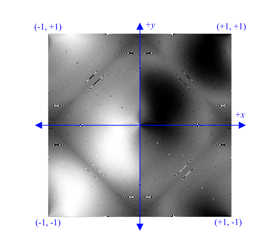
Figure 4. Optimal rounding direction for the \(y\)-component during \(float→snorm\) conversion under the precise oct encoding algorithm at 12 bits per pixel. Black = floor, white = ceiling
3.3. Packing oct24 into GL_RGB8
Like many other representations, oct24 requires underlying storage of snorm12×2 (or at least uint12×2 to emulate it), which is not supported by either CPU or GPU. Yet, this is still a desirable format in practice because it integrates directly into the space already allocated in implementations that use the popular snorm8×3 format, increasing precision without increasing storage cost. In general, packing two 12- bit values into RGB8 texture formats as unorm or uint is a desirable property.
Listing 4 shows a natural but slow method for packing the two snorm12-precision float scalars that represent oct24 into three unorm8-precision floats suitable for storage in a GL_RGB8 buffer. The required integer operations are not available on all DX9 class hardware (such as Xbox 360-generation consoles and some WebGL implementations today) and are slow compared to floating-point operations on most GPUs today. Listing 5 shows a better solution that implements the same arithmetic using only floating-point operations.
1
2
3
4
5
6
7
8
9
10
11
12
13
14
15
16
17
18
19
20
21
22
23
/* The caller should store the return value into a GL_RGB8 texture
or attribute without modification. */
vec3 snorm12x2_to_unorm8x3_slow(vec2 f) {
    // Convert to 12-bit snorm stored in a uint, using a bias (we’ll
    // reverse the bias at decode prior to division to avoid the
    // typical scaled-and-biased unorm problems)
    uint2 u = uint2(round(clamp(f, -1.0, 1.0) * 2047 + 2047));
    // Shift the bits and encode in a float, then perform unorm
    // unpacking. If storing to GL_RGB8UI, omit the division
    return vec3((u.x >> 4),
                ((u.x & 0xF) << 4) | (u.y >> 8),
                u.y & 0xFF) / 255.0;
}
vec2 unorm8x3_to_snorm12x2_slow(vec3 u) {
    // on [0, 255]
    uint3 v = uint3(u * 255.0);
    // on [0, 4095]
    uint2 p = uint2(v.x << 4) | ((v.y >> 4) & 15),
        ((v.y & 15) << 8) | v.z);
    // on [-1.0, +1.0]
    return (vec2(p) - 2047.0) / 2047.0;
}
Listing 4. Natural but slow packing of snorm12×2 data suitable for GL_RGB8 storage. We show this implementation only to explain the algorithm. Do not use this code—use Listing 5 instead.
4. Quantitative Evaluation
4.1. Accuracy
Table 1 reports the accuracy of all methods surveyed, measured on AMD and Intel 64-bit processors with \fp:strict under MSVC 2012 using float32 intermediate values for the computation and float64 values during error computation, as described below. Measurements marked with a ± suffix had substantially lower error when using float64 intermediates or different compiler flags, although we do not report those results in full because they do not occur for the high-precision methods.
For each method of representation, we measure error in terms of angular deviation between a unit float32×3 vector and the float32×3 result after encoding and then decoding. This assesses the loss of precision in the process of encoding or compressing the vector. Since we are only concerned with unit vectors, only the direction of the vector is relevant and length need not be preserved. To measure for angular error, we create one million random vectors on the unit sphere (enough so that the average angle between a vector and its closest match in the testing set is an order of magnitude lower than the precision we measure) and calculate the angular error between the original and the compressed and decompressed output. Over the set of random vectors, we compute the mean error and maximum error. Angular error is computed by converting both the input and output vectors to arrays of three doubles, normalizing them, and then taking the absolute value of the arc cosine of the dot product.
1
2
3
4
5
6
7
8
9
10
11
12
13
14
15
16
17
18
/* The caller should store the return value into a GL_RGB8 texture
or attribute without modification. */
vec3 snorm12x2_to_unorm8x3(vec2 f) {
    vec2 u = vec2(round(clamp(f, -1.0, 1.0) * 2047 + 2047));
    float t = floor(u.y / 256.0);
    // If storing to GL_RGB8UI, omit the final division
    return floor(vec3(u.x / 16.0,
                      fract(u.x / 16.0) * 256.0 + t,
                      u.y - t * 256.0)) / 255.0;
}
vec2 unorm8x3_to_snorm12x2(vec3 u) {
    u *= 255.0;
    u.y *= (1.0 / 16.0);
    vec2 s = vec2(u.x * 16.0 + floor(u.y),
                  fract(u.y) * (16.0 * 256.0) + u.z);
    return clamp(s * (1.0 / 2047.0) - 1.0, vec2(-1.0), vec2(1.0));
}
Listing 5. Optimized snorm12×2 packing into unorm8×3.
Normalization at double precision is important for accurate angle measurements. If we normalize at float32 precision during this process, the measurement error artificially appears an order of magnitude larger for 32-bit encoding methods. For 24- and 16-bit representations, the difference is negligible because the representations themselves produce significant error already.
We also evaluate every representation, computing the encoding and decoding at both float32 and float64 precision for intermediate values. Increasing the intermediate precision yields negligible change in mean or max error (less than 10−5 degrees), with the following exceptions: latlong32 maximum error increases by 1.5× using float32 instead of float64 intermediates, but the mean does not shift detectably because the additional error occurs at few locations on the sphere; the stereo, eqarea, and eqdist spherical projections when composed with the elliptical mapping to a square likewise exhibit significantly greater worst-case error at float32 intermediate precision.
| Name | Bits | Mean Error (°) | Max Error (°) |
|---|---|---|---|
| CrytekBFN24 | 24 | 0.04027 | 4.78260 |
| snorm5⇥3 | 15 | 1.45262 | 3.26743 |
| stereo+concentric16 | 16 | 0.37364 | 1.29985 |
| eqdist+concentric16 | 16 | 0.36114 | 1.05603 |
| eqarea+concentric16 | 16 | 0.36584 | 1.00697 |
| stereo16 | 16 | 0.40140 | 1.00318 |
| stereo+ellipse16 | 16 | 0.38233 | 1.00318 |
| eqarea16 | 16 | 0.38716 | 0.96092 |
| oct16 | 16 | 0.33709 | 0.94424 |
| eqarea+ellipse16 | 16 | 0.35217 | 0.90617 |
| eqdist+ellipse16 | 16 | 0.35663 | 0.79669± |
| eqdist16 | 16 | 0.38452 | 0.78944 |
| latlong16 | 16 | 0.35560 | 0.78846 |
| spherical16 | 16 | 0.35527 | 0.78685 |
| oct16P | 16 | 0.31485 | 0.63575 |
| latlong16D | 16 | 0.30351 | 0.56178 |
| snorm8⇥3 | 24 | 0.17015 | 0.38588 |
| snorm8⇥3P | 24 | 0.03164 | 0.33443 |
| stereo+concentric20 | 20 | 0.09290 | 0.32722 |
| stereo+ellipse20 | 20 | 0.09494 | 0.26171 |
| eqdist+concentric20 | 20 | 0.08975 | 0.25856 |
| stereo20 | 20 | 0.09980 | 0.24779 |
| eqarea+concentric20 | 20 | 0.09096 | 0.24671 |
| eqarea20 | 20 | 0.09627 | 0.24355 |
| oct20 | 20 | 0.08380 | 0.23467 |
| eqarea+ellipse20 | 20 | 0.08758 | 0.22567 |
| eqdist20 | 20 | 0.09541 | 0.19667 |
| eqdist+ellipse20 | 20 | 0.08851 | 0.19633 |
| spherical20 | 20 | 0.08847 | 0.19632 |
| stereo+concentric22 | 22 | 0.04642 | 0.16228 |
| oct20P | 20 | 0.07829 | 0.15722 |
| stereo+ellipse22 | 22 | 0.04746 | 0.14104 |
| eqdist+concentric22 | 22 | 0.04484 | 0.12983 |
| stereo22 | 22 | 0.04979 | 0.12437 |
| eqarea+concentric22 | 22 | 0.04545 | 0.12304 |
| eqarea22 | 22 | 0.04806 | 0.11915 |
| oct22 | 22 | 0.04180 | 0.11734 |
| eqarea+ellipse22 | 22 | 0.04374 | 0.11238 |
| eqdist+ellipse22 | 22 | 0.04418 | 0.10132 |
| spherical22 | 22 | 0.04423 | 0.09809 |
| eqdist22 | 22 | 0.04768 | 0.09806 |
| snorm10⇥3 | 30 | 0.04228 | 0.09598 |
| stereo+concentric24 | 24 | 0.02319 | 0.08305 |
| stereo+ellipse24 | 24 | 0.02372 | 0.08093± |
| oct22P | 22 | 0.03905 | 0.07898 |
| snorm11-11-10 | 32 | 0.02937 | 0.06776 |
| eqdist+concentric24 | 24 | 0.02241 | 0.06548 |
| eqarea+concentric24 | 24 | 0.02273 | 0.06265 |
| stereo24 | 24 | 0.02490 | 0.06230 |
| eqarea24 | 24 | 0.02402 | 0.06067± |
| oct24 | 24 | 0.02091 | 0.05874 |
| eqdist+ellipse24 | 24 | 0.02208 | 0.05704± |
| eqarea+ellipse24 | 24 | 0.02185 | 0.05615± |
| latlong24 | 24 | 0.02211 | 0.04907 |
| spherical24 | 24 | 0.02209 | 0.04906 |
| eqdist24 | 24 | 0.02387 | 0.04899 |
| oct24P | 24 | 0.01953 | 0.03928 |
| latlong24D | 24 | 0.01895 | 0.03504 |
| float16⇥3 | 48 | 0.00635 | 0.02635 |
| stereo+ellipse32 | 32 | 0.00149 | 0.02592± |
| eqdist+ellipse32 | 32 | 0.00138 | 0.01807± |
| eqarea+ellipse32 | 32 | 0.00137± | 0.01705± |
| spherical32 | 32 | 0.00138 | 0.00957 |
| stereo32 | 32 | 0.00155 | 0.00547± |
| stereo+concentric32 | 32 | 0.00146 | 0.00522 |
| eqdist+concentric32 | 32 | 0.00141 | 0.00409 |
| eqarea+concentric32 | 32 | 0.00142± | 0.00391 |
| eqarea32 | 32 | 0.00150 | 0.00383 |
| latlong32D | 32 | 0.00119 | 0.00381± |
| oct32 | 32 | 0.00131 | 0.00370 |
| latlong32 | 32 | 0.00138 | 0.00324± |
| eqdist32 | 32 | 0.00149 | 0.00307 |
| oct32P | 32 | 0.00122 | 0.00246 |
| snorm16⇥3 | 48 | 0.00066 | 0.00149 |
| snorm16⇥3P | 48 | 0.00060 | 0.00149 |
Table 1. Representations sorted by decreasing max error, with lines denoting a change in bit size from adjacent rows. Highlighted rows indicate techniques also implemented and evaluated on the GPU.
CPU compilers typically support up to three methods for processing high-level floating-point arithmetic: fast (fuse, distribute, and reorder operations to maximize performance), strict (store all intermediates into registers and do not reorder instructions), and precise (reorder to maximize precision, using 80-bit extended floatingpoint intermediates on some processors). In Microsoft Visual Studio these are enabled by the \fp:fast, \fp:strict, and \fp:precise compiler options. All except \fp:strict generate code that may produce different results when run on different processors.
Enhanced instruction sets (e.g., SSE and AVX) interact with these in complex ways, although we exclusively used scalar operations in our CPU experiments.
4.2. Performance
Our CPU reference implementations are reasonable, but we did not seek peak performance from them. For example, one could likely make SSE or AVX vectorized implementations with much higher throughput based on the structure of the surrounding program. We do not report timings, since performance was not a target.
We optimized the GPU implementations—which are intended for direct production use—for peak performance and report results in Table 2. The GPU decoders take floating-point values regardless of the underlying representation because texture and attribute fetches perform unorm- and snorm-to-float conversion in fixed function logic. Likewise, the encoders always return floating-point values. Our timing methodology is to encode or decode a buffer of one million unit vectors 100 times within a pixel shader, accumulating results and slightly biasing the input for each iteration to prevent the GLSL compiler from optimizing out intermediate results. We time a baseline of simply fetching and summing components and subtract that baseline from the time for each algorithm. Of course, in the context of an otherwise bandwidth- or compute-limited shader, the net ALU cost would manifest differently.
We provide some intuition for the timing results. Marketing specifications quote this GPU at about 3 teraflop/s, although that counts FMUL as two operations since it has the equivalent of 1536 scalar cores operating at 1 GHz. That indicates a theoretical maximum of 3000 fused scalar floating-point operations per nanosecond, or 1500 MUL operations. The fastest decode operation in Table 2 is spherical32, which requires 0.003680 ns per vector. That is the equivalent cost of about 5.5 scalar MUL operations per vector at the GeForce GTX 680’s theoretical maximum throughput. The decode equation comprises four trigonometric operations and two products, so the measured results appear consistent with theoretical results although they obviously depend on the architecture and may only be accurate to one significant digit for the fastest methods.
| Name | Bits | GPU Encode (ns/vector) | GPU Decode (ns/vector) |
|---|---|---|---|
| latlong32 | 32 | 0.107695 | 0.623098 |
| oct32P | 32 | 0.130082 | 0.023423 |
| oct32 | 32 | 0.023160 | 0.023341 |
| eqarea +ellipse32 | 32 | 0.020001 | 0.017153 |
| spherical32 | 32 | 0.020034 | 0.001661 |
| latlong24 | 24 | 0.097284 | 0.045110 |
| oct24P | 24 | 0.134439 | 0.030122 |
| oct24 | 24 | 0.026816 | 0.030102 |
| eqarea +ellipse24 | 24 | 0.027087 | 0.017230 |
| spherical24 | 24 | 0.022747 | 0.001904 |
| snorm8×3P | 24 | 1.135096 | 0.001888 |
| CrytekBFN24 | 24 | 0.574226 | 0.001887 |
| latlong16 | 16 | 0.068668 | 0.033396 |
| oct16P | 16 | 0.129718 | 0.023333 |
| oct16 | 16 | 0.023132 | 0.023384 |
| eqarea +ellipse16 | 16 | 0.020020 | 0.017153 |
| spherical16 | 16 | 0.020027 | 0.001656 |
Table 2. GPU encode and decode times for the highest quality methods at various precisions, as measured on NVIDIA GeForce GTX 680 (Kepler architecture).
4.3. Representable Point Distribution - 代表点分布
To understand the maximum error, we show the distribution on the sphere of all representable points for each format at net 16 bit precision. For comparison, we also show the 24-bit snorm×3 distribution, which is very poor compared to even the 16- bit alternatives. Recall that an ideal representation will produce a uniform distribution of points and that the darker areas in this figure indicate areas that are biased towards lower error, while the lighter areas represent regions of higher error. For any particular vector, the error depends on the exact local distribution, however.
4.4. Qualitative Evaluation - 定性评价
The primary concern for a graphics application is often not quantitative representation error but how perceptible the artifacts are in the final image that manifest as a result of that error. Thus, while it is important to quantify the surveyed representations, an implementor will often make a final design decision based on an image.
Image quality as a function of unit vector representation depends on how the unit vectors are applied in the rendering pipeline, the lighting conditions, and the materials and geometry involved. For example, a scene with bumpy, glossy surfaces lit by photon mapping is likely to be more sensitive to representation error in per-pixel surface normals than to representation error in per-vertex tangent vectors, and far less sensitive to representation error in incident photon directions.
One reasonable qualitative metric is the smoothness and accuracy of the shading as the surface normal representation changes. We created a scene with a mixture of curvy, polygonal, and bumpy objects and rendered it with three reflectance models: Lambertian, glossy, and mirror reflective. We use deferred shading with the normals encoded in the G-buffer, which introduces per-pixel representation error. The mirror reflective curvy object is the one that is most sensitive to normal representation error. We show images with the three reflectance models for the methods that we optimized for the GPU, since those are the ones most interesting for practical application. For each, we consider 16-, 24-, and 32-bit net variants and precise variants where relevant.
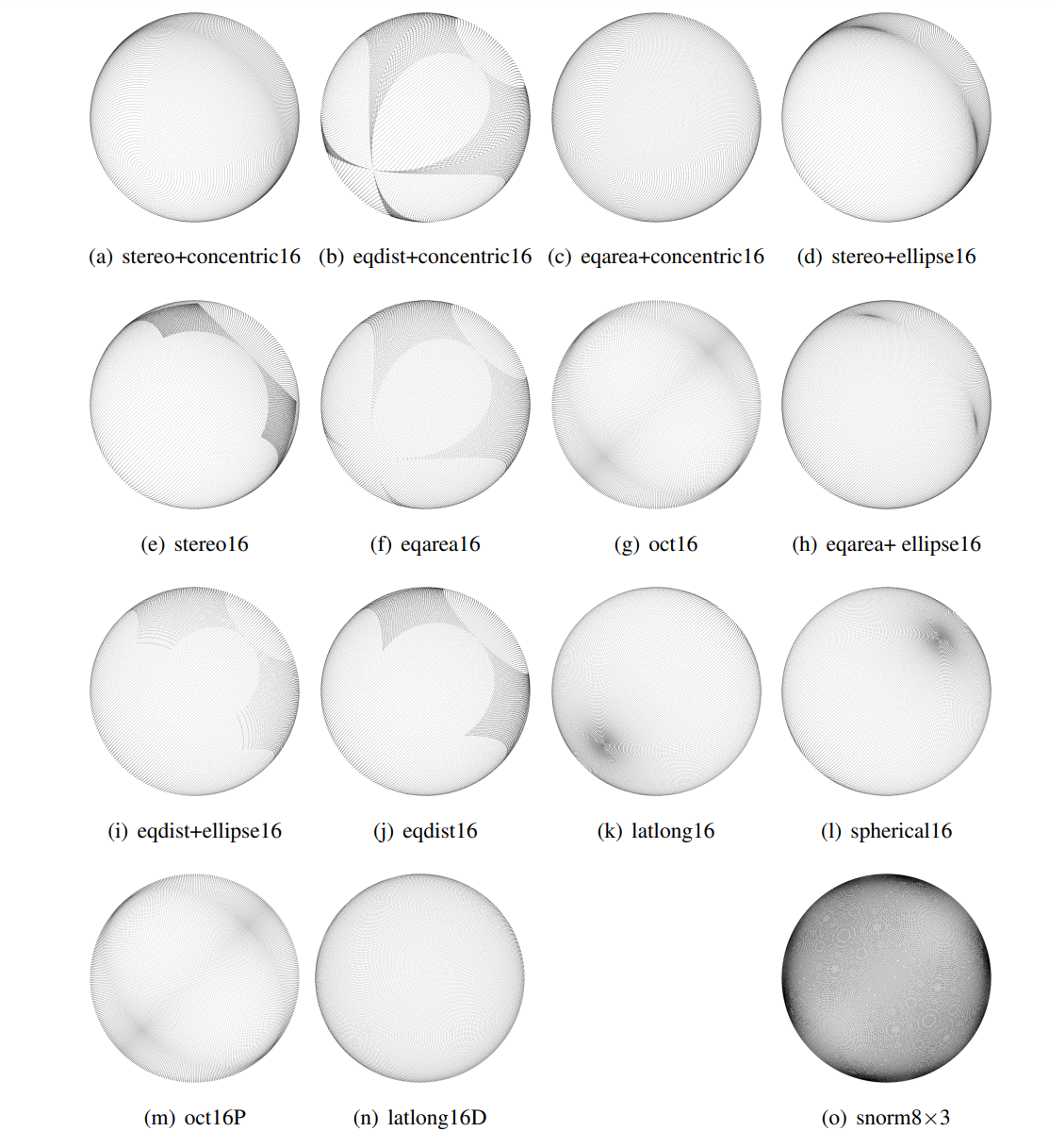
Figure 5. Distribution of representable unit vectors at 16-bit precision, with 24-bit snorm8×3 added for comparison. 24- and 32-bit representations yield distributions too dense to visualize effectively at this scale. Darker areas represent regions of lower error.
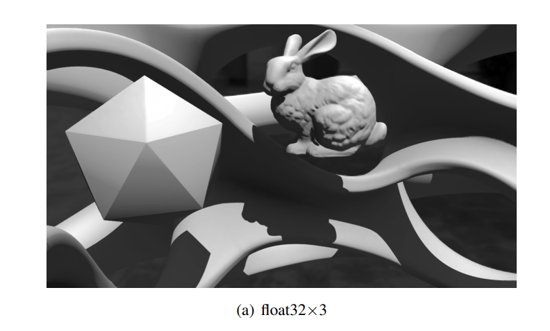
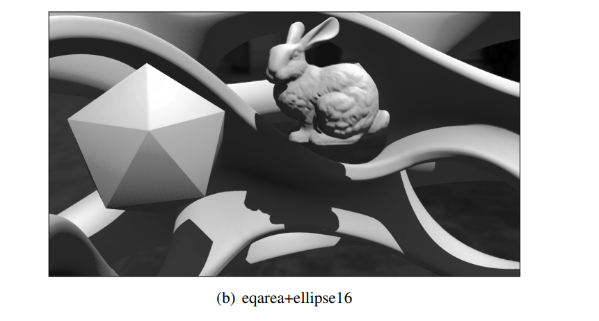
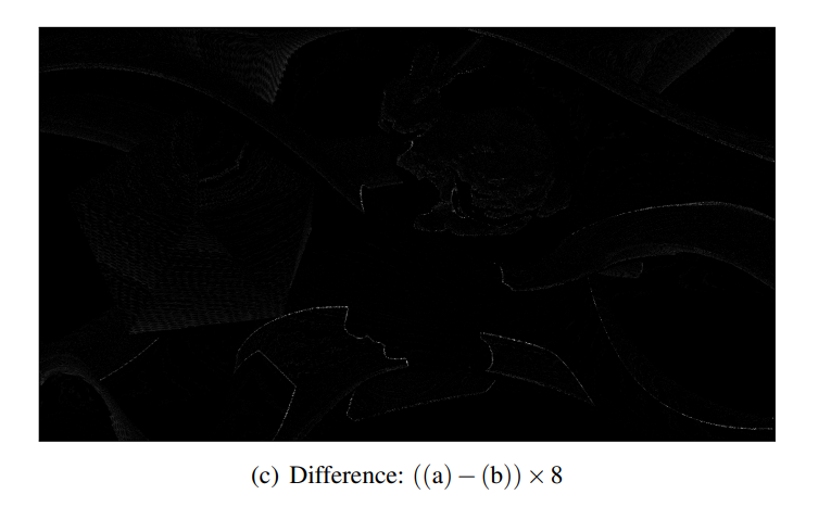
Figure 6. Normal representations yield minimal differences in shading under a Lambertian BRDF, even comparing the implemented GPU representation with the highest mean error to float32×3. See the supplementary materials for images generated with all of the implemented GPU methods.

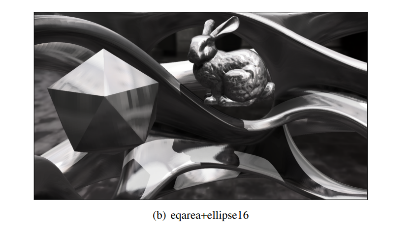
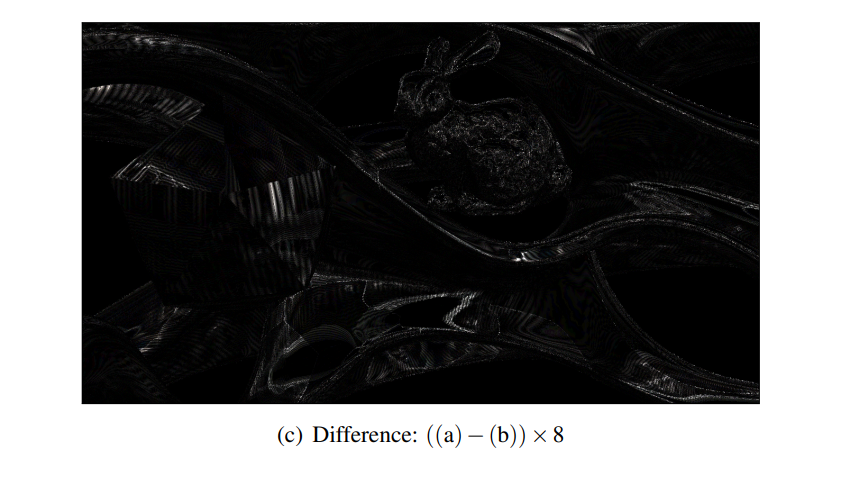
Figure 7. Differences in shading are far more apparent under a glossy BRDF than under a Lambertian one. Discretization is visible on nearly flat surfaces and the 8× difference image reveals moderate error in eqarea+ellipse16. See the supplementary materials for a comparison with all implemented methods.
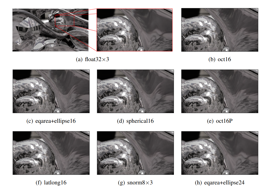
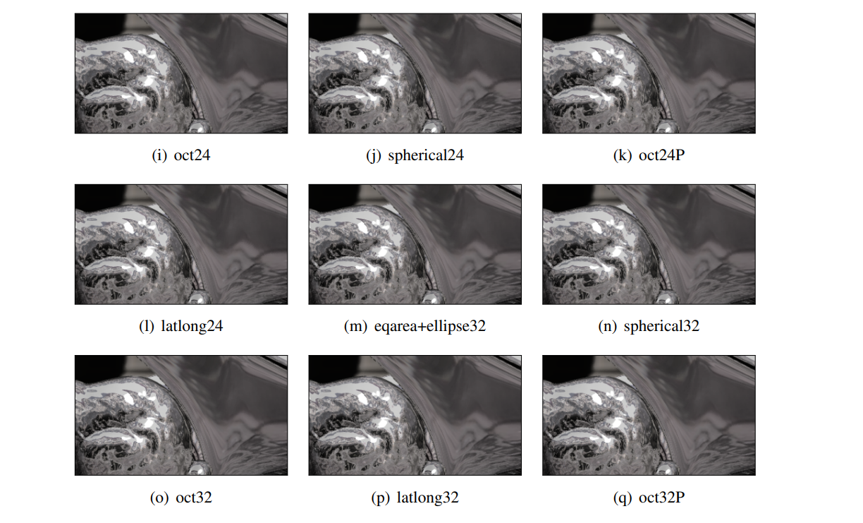
Figure 8. Various normal representations yield significant differences in shading under a mirror BRDF. See the supplementary materials for the full uncropped images and corresponding difference images.
5. Conclusions and Future Work
The oct and spherical representations are clearly the most practical. They are close to minimal error among the surveyed methods and have very efficient implementations that require no tables.
Spherical has better decode speed than oct on the tested architecture, and oct has slightly better quality and encode speed. For low bit sizes, the precise oct variant gives significantly better quality. The oct mapping is sufficiently simple and stateless that we suggest future graphics APIs provide a hardware abstraction of oct32 attribute and texture formats, with future GPUs then able to support texture and attribute fetch (and framebuffer and attribute write) in fixed-function hardware, akin to sRGB, to eliminate the remaining time cost.
When perception of error—particularly shading error—is more important than actual error, we suggest that adding a little noise during either encoding or decoding based on the known mean error of the method would help to break up the quantization artifacts arising from limited precision. We observe that Crytek’s implementation of snorm8×3P does this in Crysis 2, albeit not in a controlled fashion. The open challenge is to add noise in a way that is somewhat temporally coherent under animation and does not increase mean error
There are several places in a GPU pipeline where one might wish to encode a 3D unit vector to reduce memory resource demands: vertex attributes, interpolators, normal maps, and geometry buffers. We explicitly focused on storage of spatially independent vectors, which implicitly means vertex attributes and geometry buffers, in our work. We do not recommend compressing interpolators; the octahedral format was designed for storage, not computation, and although it will interpolate linearly with small amounts of error over small distances away from the boundaries of the unit square, we have not found that error and the complexity of handling boundaries to be justified even by a 3x bandwidth/register size reduction for interpolators.
Low-frequency normal maps benefit from spatial compression in formats like DXN, and the additional gain from switching to oct is likely to be modest at best. For high-frequency normal maps, it would be interesting to explore the use of oct as a compressed format, since DXN will produce large error (it has a fixed compression ratio) in this case. One nice but important limitation of doing so is that oct eliminates the redundant information of the normal’s length, so, for example, the common use of Toksvig’s method [Toksvig 2005] of using the MIP-mapped normal’s reduced length as an inexpensive metric for surface normal variance does not apply—this information has to be explicitly stored. We note that rotating and scaling the standard oct encoding so that the +Z hemisphere covers the unit square in parameter space adds few operations and eliminates the branch in the encoding function, while doubling the number of bit patterns used to encode the hemisphere (see Listing 6). In Table 3, we compare this “hemi-oct” encoding to storing only the X- and Y-components of the original unit vector, which is an encoding scheme used in several tangent-space normal map compression algorithms[van Waveren and Castaño 2008]. Hemi-oct has significantly less mean and max error than the xy-only encoding, over uniformly distributed unit vectors in the +Z hemisphere. We note this as a promising area for future research.
1
2
3
4
5
6
7
8
9
10
11
12
13
14
15
// Assume normalized input on +Z hemisphere.
// Output is on [-1, 1].
vec2 float32x3_to_hemioct(in vec3 v) {
    // Project the hemisphere onto the hemi-octahedron,
    // and then into the xy plane
    vec2 p = v.xy * (1.0 / (abs(v.x) + abs(v.y) + v.z));
    // Rotate and scale the center diamond to the unit square
    return vec2(p.x + p.y, p.x - p.y);
}
vec3 hemioct_to_float32x3(vec2 e) {
    // Rotate and scale the unit square back to the center diamond
    vec2 temp = vec2(e.x + e.y, e.x - e.y) * 0.5;
    vec3 v = vec3(temp, 1.0 - abs(temp.x) - abs(temp.y));
    return normalize(v);
}
Listing 6. Fast \(float32×3 → hemi—oct\) variant and its inverse for any bit size
| Name | Bits | Mean Error (◦) | Max Error (◦) |
|---|---|---|---|
| XYOnly16 | 16 | 0.46669 | 5.71419 |
| XYOnly32F | 32 | 0.07759 | 2.10047 |
| XYOnly24 | 24 | 0.03844 | 1.43251 |
| oct16P | 16 | 0.31485 | 0.63574 |
| HemiOct16 | 16 | 0.24000 | 0.55112 |
| XYOnly32 | 32 | 0.00298 | 0.35281 |
| oct24P | 24 | 0.01953 | 0.03928 |
| HemiOct24 | 24 | 0.01489 | 0.03406 |
| oct32P | 32 | 0.00122 | 0.00246 |
| HemiOct32 | 32 | 0.00093 | 0.00213 |
Table 3. The hemi-oct format encodes unit vectors on the hemisphere with significantly more accuracy than the standard xy-only encoding, and even improves substantially upon the precise oct variant at equivalent bit sizes. These values were computed over one million vectors uniformly chosen over the hemisphere.
We have exclusively considered 3D unit vectors. What about other dimensions? It takes only one bit to encode the two possible 1D unit vectors, -1 and +1. 2D unit vectors are trivially space-optimally encoded by a fixed point (scaled by 2π). In 4D, it would be desirable to encode unit quaternions using a 4D analog of the oct format, however, the symmetries are much more complex and it does not scale easily or obviously.
For many applications (e.g., normal maps, G-buffers), it is important to have high precision on only half of the sphere and relatively low precision can be assigned to the other half. For example, in a G-buffer, most surface normals point towards the camera. One approach suggested to us by Peter-Pike Sloan is to use the oct encoding, but distort the unit square before the final mapping to snorm during encoding.
Ref : Survey of Efficient Representations for Independent Unit Vectors